Introducing Decomps and Due-Tos
Neal Fultz <neal@njnm.consulting>
for System1
Tue, Aug 25, 2020
bit.ly/3goPBJk
Executive Summary
Decompositions and Dueto reports are extremely useful for
- understanding which variables are contributing to outcomes of interest (eg Sales)
- how that contribution is changing over time
- by approximating, summarizing and aggregating sets of linear effects
They are typically presented as bar or waterfall charts.
Because it measures all contributions on the same units (dollars) and can be arbitrarily aggregated, they are much easier to interpret than raw regression results.
Modern software can calculate them automatically.
Disclaimer
The most striking thing about the business world is its jargon. It does not have a monopoly on this, since we live in a world of claptrap. Universities, the media, and psychoanalysts are masters of the genre. Still, business jargon is particularly deadly, enough to utterly discourage the workplace hero, the Stakhanovite, lying dormant in you. -- Corinne Maier
What are Decompositions and why should I care?
what
the state or process of rotting; decay.- to separate into constituent parts or elements or into simpler compounds
why
- simpler parts are easier to understand
- reason about how parts interact with each other and with system as a whole
commonly used
- Marketing - attribute sales to different channels
- Cost Accounting - direct vs indirect, fixed vs variable
- Chemistry - literally break down a complex molecule into atoms
- Math - Factoring split a natural number into it's primes
- Stats - Fisher's ANOVA - split variance into between / Within
Calculus Refresher 1 - Taylor's Theorem
Taylor approximation the other direction
Vector notation: $$ f(x_{k}) = a + x'L + h(x) $$
Taylor, so what?
"best" "linear" "additive" "decomposition" of "Y into X"
Implementing the OLS Decomp
... just don't add the columns together. eg cross out the $1$.
Interpreting a Decomp, theory
Comments
- Same shape as $X$ ($\pm$ error term).
- Same units as $Y$.
- "Grounds" "contribution" of each "input" to common scale
- Think about which X you can control / manipulate.
Linear Aggregation
- Can left multiply $A\mbox{ decomp}(Y)$ to calculate summary stats.
- In practice, equivalent to a
SUM() / GROUP BY
- In practice, equivalent to a
- By choosing A carefully
- $A'e = 0 \rightarrow A \mbox{ decomp} (Y) = A \mbox{ decomp} (\hat{Y})$
- In OLS, residuals sum to 0 (eg $1'e = 0$
- Totals: $A = 1'_n$ : Totals
- Means: $A = \frac{1}{n} 1'_n$: Mean
- Group Breakouts: $A = \mbox{dummy}(G)$
- If $G \in X$, $Ge = 0$
- By assoc, can group $(AX)\hat\beta$, use as contrasts for hypothesis testing.
- Reports can "drill down" to same unit of observation as underlying data.
- Y follows "accounting", all errors cancel
Calculus Refresher 2 - Chain Rule
what if slopes also vary by t
$$ \frac{\partial}{\partial t } f(t) g(t) = \frac{\partial f}{\partial t } g(t) + f(t) \frac{\partial g}{\partial t }$$$$ \frac{\partial}{\partial t }Y = \alpha + \frac{\partial X_1}{\partial t } \beta_1 + X_1 \frac{\partial \beta_1}{\partial t } + \frac{\partial X_2}{\partial t } \beta_2 + X_2 \frac{\partial \beta_2}{\partial t } + \dots + \epsilon $$Non Linear Models (advanced)
If not using OLS, the above is not justified.
But, combining taylor expansion + chain rule for each element of Y:
$$ y_i = a + \sum x_i \frac{\partial y}{\partial x_i}|_0 + h(x) $$And back to matrix notation: $$ Y = (X \circ \nabla Y) 1_k + h(X) $$
Where $\circ$ is the Hadamard product and $\nabla Y$ is the deriviative of Y wrt to X.
Note: Error term not "nice" anymore. Many (mostly ad-hoc) methods for dealing with them.
Non Linear Models (Historical Digression)
Note: Instead of dealing with $\nabla Y$ analytically (annoying and/or hard), use modern software to carry out procedure numerically.
- In ancient times, you would hire an economist to work this analytically on a yellow pad, and a programmer to translate that to custom software.
- In the recent past, replace the economist with wolfram alpha.
- In present day, replace the programmer with auto diff.
What are Duetos and why should I care?
what
- sadly, not dictionary word.
- "How did an output change (over time) in relation to how it's inputs changed (over time)"
why
- Complicated systems change in complicated ways
common uses
- Time Series
- A/B testing
Implementing Duetos
if time/treatment is modeled explicitly
- then could analytically chain rule through.
- this yields calculus / "smooth" result
- applies to time series models with a trend variable, for example.
- do we even want this?
if time/treatment is contained within row space...
lets back up, go left at Alburque
$$ \frac{\partial f}{\partial t} = \lim_{dt \to 0} \frac{f(x, t + dt) - f(x, t)}{t + dt - t} \approx \frac{f(x, t:=1) - f(x, t:=0)}{1 - 0} $$ $$ \approx I(t=1) \mbox{ decomp} (Y) - I(t=0) \mbox{ decomp} (Y) $$ $$ \approx [I(t=1) - I(t=0)] \mbox{ decomp} (Y) $$
- So let $A = [I(t=1) - I(t=0)]$
- then duetos can be approximated by linear aggregation of the decomp.
- which subtracts, from a target group, a base group (eg A/B testing, YoY analyses, ...)
- Caveat Be careful about totals vs means, and propagate error terms carefully.
Example - LA DWP
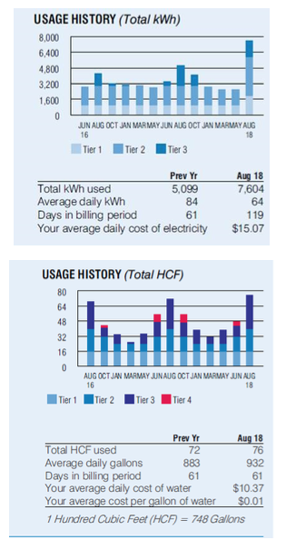
Why is my power bill so high and inconsistent?
Theory 1: "My Fault" / Demand
- Heating / Cooling
- Heating is basically electric blanket in ceiling, is stupid
- Cooling is window units, replaced in 2019
- Depends on temperature outside?
- Appliances
- Turtle Tank filter -> big upgrade ~ 2017
- Aero Garden (new after Xmas 2019)
- Curliecue light bulbs (cycling in since 2011)
- Newer computers have lower power draw, replaced 2019
Why is my power bill so high and inconsistent?
Theory 2: "Their Fault" / Supply
- Seasonal changes in supply
- Less solar in winter months?
- Backfill extra summer demand with more expensive engergy?
- Inflation?
- Changes in city ordinances?
- ladwpbillingsettlement.com
The LADWP may owe another $40 million to consumers after overcharging them years. The FBI raided the LADWP and City Attorney's offices last Monday investigating, bribery, kickbacks, extortion and money laundering. Consumer Watchdog President Jamie Court says there is no doubt crimes were committed and that the consumers are owed millions.
Data
- LA DWP Bimonthly Bills
- 2016 - Present
- Progressive pricing by tier
- higher tiers not reported unless used
- Days per billing cycle can vary from 57 - 64
- Inflation
- BLS CPI data
- Series CUUR0400SEHF / Energy services in West urban, all urban consumers, not seasonally adjusted
- Climate
- Weather Underground KLAX station
- Use middle month avg temp - eg for Dec 15-Feb 13 bill, use Jan
Data
Data

Data

Modeling Tier 1 Price
Plotting
decomp = X.apply(lambda x: x * results.params[x.name])

Plotting (Stacked)

Back transform to Dollars, get rid of log
- We want to not be on log scale
- Back transforming is a nonlinear function, $e^\hat{y}$
- Chain rule: $ \frac{\partial}{\partial x_i} e^\hat{y} = e^\hat{y} \beta_i$
- Back transforming is a nonlinear function, $e^\hat{y}$
decomp = X.apply(lambda x: x * numpy.exp(results.fittedvalues) * results.params[x.name])
- ¡Extra Caution with base bucket!
- Log Normal - add back $\sigma^2/2$
decomp.head()
Plotting (dollar scale)

Plotting (Stacked)

Linear Aggregation
- Multiply decomposed price components by actual usage
- Aggregate to yearly level
yearly_decomp = ( decomp.drop(columns="yyyymm").
      multiply(df['usage'], axis='index').
      groupby(df['yyyy']).
      mean())

Year-over-Year Dueto
- Multiply decomposed price components by actual usage
- Aggregate to yearly level
yoy_dueto = yearly_decomp.loc[4] - yearly_decomp.loc[3]

Plotting Duetos

Dealing with Usage
- Those decomps take usage as a given / "fixed".
- But what if usage is also being changed by some underlying process?
- Which implies we should have chained those effects through both Price and Usage.
- That algebra is not fun. :(
- Instead, we can evaluate the deriviatives numerically using keras, and construct decomps from those.
- If taking this route, may as well let it figure out how to parameterize features.
def log_log_builder():
    model = Sequential([
      Lambda(tensorflow.keras.backend.log),
      Dense(DIM, input_shape=(X.shape[1], ), kernel_initializer='normal', activation='relu'),
      Dense(Y.shape[1]),
      Lambda(tensorflow.keras.activations.exponential, output_shape=[2])
    ])
    model.compile(loss=scaled_mse, optimizer='adam')
    return model
estimator = KerasRegressor(build_fn=log_log_builder, epochs=10000, batch_size=20, verbose=0)

estimator.fit(X, Y)
yhat = estimator.predict(X,)

Extracting derivs numerically
with tensorflow.GradientTape() as tape:
    Xk = tensorflow.keras.backend.constant(X, shape=X.shape)
    tape.watch(Xk)
    yhat = estimator.model(Xk[:,:])
derivs = tape.jacobian(yhat, Xk)
derivs = derivs.numpy()
Total Bill via Keras
total_bill = KerasRegressor(lambda: None)
total_bill.model = Sequential( estimator.model.layers[:-1] + [
    Lambda(lambda x: tensorflow.keras.activations.exponential(x[:,0] + x[:,1]), output_shape=[1])
  ])

Duetos (Keras)
decomp_bill = (derivs * X).groupby(df['yyyy']).mean()
dueto_keras = decomp_bill.loc[2020] - decomp_bill.loc[2019]

Executive Summary
Decompositions and Dueto reports are extremely useful for
- understanding which variables are contributing to outcomes of interest (eg Sales)
- how that contribution is changing over time
- by approximating, summarizing and aggregating sets of linear effects
They are typically presented as bar or waterfall charts.
Because it measures all contributions on the same units (dollars) and can be arbitrarily aggregated, they are much easier to interpret than raw regression results.
Modern software can calculate them automatically.
# Questions ?
Q: Who are you?
- Former SWE / RSE in CPG => Data Science in Lending, AdTech (+mobile)
- Grad school at Berkeley iSchool, UCLA Stats
- Part-time stats consultant since 2007, went independent in 2019
- Contributor to R, Jupyter, GNU Screen, ...
- Mentor on SharpestMinds, Springboard, MentorCruise, ...
- Add me on LinkedIn and GitHub
Q: Where did duetos come frome?
This is a great question that I don't have a good answer for.
Additive decompositions have been in Mathematics for a long time, but in the modern sense, popped up in Economics in the postwar era as people tried to figure out how inflation indexes were behaving, and then spread to psychology via quantitative marketing.
For Duetos, it's unclear unclear to me who invented them, who named them, or when or where; I learned on the job at a company with ex-Deloitte founders.
Q: What is the relationship of Decomps with Explainability / Fairness?
In Explanability / Fairness, decompose "contribution" for a specific point for each variable, by inspecting the partial (directional) derivative at the point.
Decomps and duetos take the derivative at the reference group / origin / time 0 for all points and aggregate.
Q: Any practice problems / extensions?
Easy: Propogate error, incorporate into plots
Medium: Extend the keras model to incorporate Tier 2 and Tier 3 pricing. (Hint: Use ReLU layers)
Medium: Incorporate time series components into trend, seasonality as in Hyndman
Impossible: Interpret cable bill
Q: How to account for "error bucket" / model bias?
In OLS, if you have any Y error remaining and unallocated, add the group to the set of predictors.
For the nonlinear case, the easiest way is calculate the residual, and carry it around.
Q: How to account for "error bars" / model uncertainty?
- Don't do this for waterfall plots / other cumed plots; the CIs may mislead, will understate cumulative uncertainty
- In OLS, the std errors are probably fine
- In the nonlinear setting, you will need to resort to the bootstrap.
- consider Bayesian bootstrap, it can preserve panel structure.
Q: How about doing decomps as pie charts?
- FFS
- Serious answer - decomps can go negative, and you can't have a negative slice.
Q: How to deal with negative buckets?
- Just like you can center variables without affecting slopes, you can slide them such that their minimum is zero.
- Be very careful when aggregating over buckets that have both positive and negative values, they will cancel out.
- If you are going the numerical route, consider
log1pand other sign preserving transforms and activation functions. - In a stacked bar chart, you should split out and plot the negatives seperately.
- Don't use Red/Green pairs to indicate the sign though.
Q: How about interactive visualizations?
- +1 - R Shiny is good for this. D3 can work but push computation to an API.
- For Decomps, you need ways to specify the scope of the base group.
- Duetos will also need to specify the alternative group.
Q: How did you make these slides?
- Jupyter Notebook - Programming environment
- plotnine - a grammar of graphics in python
- statsmodels - common statistical models
- keras - easy(er) n-nets
- reveal.js - HTML5 presentation
Q: How did you get branding on the slides?
Jupyter Lab does not embed custom.css (issue 8793), but you can manually dump style rules into
the notebook.
from IPython.core.display import display, HTML
display(HTML(f'<style>{_css}</style>'))
For logos, use base64 dataurls inside the CSS.